# install the latest version of the Epi R Handbook package
pacman::p_install_gh("appliedepi/epirhandbook")2 Download handbook and data
2.1 Download offline handbook
You can download the offline version of this handbook as an HTML file so that you can view the file in your web browser even if you no longer have internet access. If you are considering offline use of the Epi R Handbook here are a few things to consider:
- When you open the file it may take a minute or two for the images and the Table of Contents to load
- The offline handbook has a slightly different layout - one very long page with Table of Contents on the left. To search for specific terms use Ctrl+f (Cmd-f)
- See the Suggested packages page to assist you with installing appropriate R packages before you lose internet connectivity
- Install our R package epirhandbook that contains all the example data (install process described below)
There are two ways you can download the handbook:
Use download link
For quick access, right-click this link and select “Save link as”.
If on a Mac, use Cmd+click. If on a mobile, press and hold the link and select “Save link”. The handbook will download to your device. If a screen with raw HTML code appears, ensure you have followed the above instructions or try Option 2.
Use our R package
We offer an R package called epirhandbook. It includes a function download_book() that downloads the handbook file from our Github repository to your computer.
This package also contains a function get_data() that downloads all the example data to your computer.
Run the following code to install our R package epirhandbook from the Github repository appliedepi. This package is not on CRAN, so use the special function p_install_gh() to install it from Github.
Now, load the package for use in your current R session:
# load the package for use
pacman::p_load(epirhandbook)
Next, run the package’s function download_book() (with empty parentheses) to download the handbook to your computer. Assuming you are in RStudio, a window will appear allowing you to select a save location.
# download the offline handbook to your computer
download_book()
2.2 Download data to follow along
To “follow along” with the handbook pages, you can download the example data and outputs.
Use our R package
The easiest approach to download all the data is to install our R package epirhandbook. It contains a function get_data() that saves all the example data to a folder of your choice on your computer.
To install our R package epirhandbook, run the following code. This package is not on CRAN, so use the function p_install_gh() to install it. The input is referencing our Github organisation (“appliedepi”) and the epirhandbook package.
# install the latest version of the Epi R Handbook package
pacman::p_install_gh("appliedepi/epirhandbook")
Now, load the package for use in your current R session:
# load the package for use
pacman::p_load(epirhandbook)
Next, use the package’s function get_data() to download the example data to your computer. Run get_data("all") to get all the example data, or provide a specific file name and extension within the quotes to retrieve only one file.
The data have already been downloaded with the package, and simply need to be transferred out to a folder on your computer. A pop-up window will appear, allowing you to select a save folder location. We suggest you create a new “data” folder as there are about 30 files (including example data and example outputs).
# download all the example data into a folder on your computer
get_data("all")

# download only the linelist example data into a folder on your computer
get_data(file = "linelist_cleaned.rds")
# download a specific file into a folder on your computer
get_data("linelist_cleaned.rds")Once you have used get_data() to save a file to your computer, you will still need to import it into R. see the Import and export page for details.
If you wish, you can review all the data used in this handbook in the “data” folder of our Github repository.
Download one-by-one
This option involves downloading the data file-by-file from our Github repository via either a link or an R command specific to the file. Some file types allow a download button, while others can be downloaded via an R command.
Case linelist
This is a fictional Ebola outbreak, expanded by the handbook team from the ebola_sim practice dataset in the outbreaks package.
Click to download the “raw” linelist (.xlsx). The “raw” case linelist is an Excel spreadsheet with messy data. Use this to follow-along with the Cleaning data and core functions page.
Click to download the “clean” linelist (.rds). Use this file for all other pages of this handbook that use the linelist. A .rds file is an R-specific file type that preserves column classes. This ensures you will have only minimal cleaning to do after importing the data into R.
Other related files:
Part of the cleaning page uses a “cleaning dictionary” (.csv file). You can load it directly into R by running the following commands:
pacman::p_load(rio) # install/load the rio package

# import the file directly from Github
cleaning_dict <- import("https://github.com/appliedepi/epirhandbook_eng/raw/master/data/case_linelists/cleaning_dict.csv")
Malaria count data
These data are fictional counts of malaria cases by age group, facility, and day. A .rds file is an R-specific file type that preserves column classes. This ensures you will have only minimal cleaning to do after importing the data into R.
Likert-scale data
These are fictional data from a Likert-style survey, used in the page on Demographic pyramids and Likert-scales. You can load these data directly into R by running the following commands:
pacman::p_load(rio) # install/load the rio package

# import the file directly from Github
likert_data <- import("https://raw.githubusercontent.com/appliedepi/epirhandbook_eng/master/data/likert_data.csv")
Flexdashboard
Below are links to the file associated with the page on Dashboards with R Markdown:
Contact Tracing
The Contact Tracing page demonstrated analysis of contact tracing data, using example data from Go.Data. The data used in the page can be downloaded as .rds files by clicking the following links:
Click to download the case investigation data (.rds file)
Click to download the contact registration data (.rds file)
Click to download the contact follow-up data (.rds file)
NOTE: Structured contact tracing data from other software (e.g. KoBo, DHIS2 Tracker, CommCare) may look different. If you would like to contribute alternative sample data or content for this page, please contact us.
TIP: If you are deploying Go.Data and want to connect to your instance’s API, see the Import and export page (API section) and the Go.Data Community of Practice.
GIS
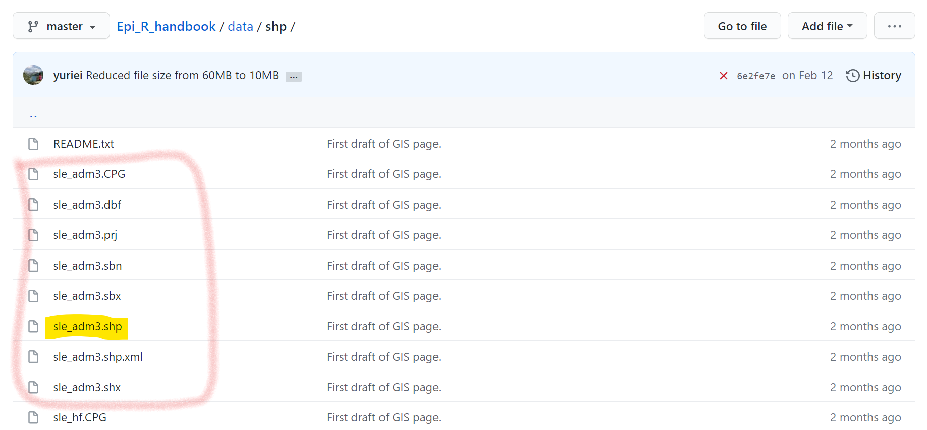
Shapefiles have many sub-component files, each with a different file extention. One file will have the “.shp” extension, but others may have “.dbf”, “.prj”, etc.
The GIS basics page provides links to the Humanitarian Data Exchange website where you can download the shapefiles directly as zipped files.
For example, the health facility points data can be downloaded here. Download “hotosm_sierra_leone_health_facilities_points_shp.zip”. Once saved to your computer, “unzip” the folder. You will see several files with different extensions (e.g. “.shp”, “.prj”, “.shx”) - all these must be saved to the same folder on your computer. Then to import into R, provide the file path and name of the “.shp” file to st_read() from the sf package (as described in the GIS basics page).
If you follow Option 1 to download all the example data (via our R package epirhandbook), all the shapefiles are included.
Alternatively, you can download the shapefiles from the R Handbook Github “data” folder (see the “gis” sub-folder). However, be aware that you will need to download each sub-file individually to your computer. In Github, click on each file individually and download them by clicking on the “Download” button. Below, you can see how the shapefile “sle_adm3” consists of many files - each of which would need to be downloaded from Github.
Phylogenetic trees
See the page on Phylogenetic trees. Newick file of phylogenetic tree constructed from whole genome sequencing of 299 Shigella sonnei samples and corresponding sample data (converted to a text file). The Belgian samples and resulting data are kindly provided by the Belgian NRC for Salmonella and Shigella in the scope of a project conducted by an ECDC EUPHEM Fellow, and will also be published in a manuscript. The international data are openly available on public databases (ncbi) and have been previously published.
- To download the “Shigella_tree.txt” phylogenetic tree file, right-click this link (Cmd+click for Mac) and select “Save link as”.
- To download the “sample_data_Shigella_tree.csv” with additional information on each sample, right-click this link (Cmd+click for Mac) and select “Save link as”.
- To see the new, created subset-tree, right-click this link (Cmd+click for Mac) and select “Save link as”. The .txt file will download to your computer.
You can then import the .txt files with read.tree() from the ape package, as explained in the page.
ape::read.tree("Shigella_tree.txt")Standardization
See the page on Standardised rates. You can load the data directly from our Github repository on the internet into your R session with the following commands:
# install/load the rio package
pacman::p_load(rio)

##############
# Country A
##############
# import demographics for country A directly from Github
A_demo <- import("https://github.com/appliedepi/epirhandbook_eng/raw/master/data/standardization/country_demographics.csv")

# import deaths for country A directly from Github
A_deaths <- import("https://github.com/appliedepi/epirhandbook_eng/raw/master/data/standardization/deaths_countryA.csv")

##############
# Country B
##############
# import demographics for country B directly from Github
B_demo <- import("https://github.com/appliedepi/epirhandbook_eng/raw/master/data/standardization/country_demographics_2.csv")

# import deaths for country B directly from Github
B_deaths <- import("https://github.com/appliedepi/epirhandbook_eng/raw/master/data/standardization/deaths_countryB.csv")


###############
# Reference Pop
###############
# import demographics for country B directly from Github
standard_pop_data <- import("https://github.com/appliedepi/epirhandbook_eng/raw/master/data/standardization/world_standard_population_by_sex.csv")
Time series and outbreak detection
See the page on Time series and outbreak detection. We use campylobacter cases reported in Germany 2002-2011, as available from the surveillance R package. (nb. this dataset has been adapted from the original, in that 3 months of data have been deleted from the end of 2011 for demonstration purposes)
Click to download Campylobacter in Germany (.xlsx)
We also use climate data from Germany 2002-2011 (temperature in degrees celsius and rain fail in millimetres) . These were downloaded from the EU Copernicus satellite reanalysis dataset using the ecmwfr package. You will need to download all of these and import them with stars::read_stars() as explained in the time series page.
Click to download Germany weather 2002 (.nc file)
Click to download Germany weather 2003 (.nc file)
Click to download Germany weather 2004 (.nc file)
Click to download Germany weather 2005 (.nc file)
Click to download Germany weather 2006 (.nc file)
Click to download Germany weather 2007 (.nc file)
Click to download Germany weather 2008 (.nc file)
Click to download Germany weather 2009 (.nc file)
Survey analysis
For the survey analysis page we use fictional mortality survey data based off MSF OCA survey templates. This fictional data was generated as part of the “R4Epis” project.
Click to download Fictional survey data (.xlsx)
Shiny
The page on Dashboards with Shiny demonstrates the construction of a simple app to display malaria data.
To download the R files that produce the Shiny app:
You can click here to download the app.R file that contains both the UI and Server code for the Shiny app.
You can click here to download the facility_count_data.rds file that contains malaria data for the Shiny app. Note that you may need to store it within a “data” folder for the here() file paths to work correctly.
You can click here to download the global.R file that should run prior to the app opening, as explained in the page.
You can click here to download the plot_epicurve.R file that is sourced by global.R. Note that you may need to store it within a “funcs” folder for the here() file paths to work correctly.

